More protein dynamics with ProDy

Original slides courtesy Ahmet Bakan

print view
notebook

Dynamics Analysis

ProDy can be used for

• Principal component analysis (PCA) of
  • NMR models
  • X-ray ensembles
  • Homologous structure ensembles
• Essential dynamics analysis (EDA) of trajectories
• Anisotropic and Gaussian network model (ANM/GNM) calculations
• Analysis of normal mode data from external programs

PCA calculations

Let’s perform principal component analysis (PCA) of an ensemble of NMR models, such as 2k39. First, we prepare an ensemble:

from prody import *
import py3Dmol
ubi = parsePDB('2lz3')
print(ubi.numCoordsets())

showProtein(ubi)

Minimize the differences between each structure...

ubi_ensemble = Ensemble(ubi.calpha)
print("Before iterpose",ubi_ensemble.getRMSDs().mean())
ubi_ensemble.iterpose()
print("After iterpose",ubi_ensemble.getRMSDs().mean())

help(ubi_ensemble.iterpose)

What is PCA?

Principal component analysis (PCA) is a statistical procedure that uses an orthogonal transformation to convert a set of observations of possibly correlated variables into a set of values of linearly uncorrelated variables called principal components. The number of principal components is less than or equal to the number of original variables. This transformation is defined in such a way that the first principal component has the largest possible variance (that is, accounts for as much of the variability in the data as possible), and each succeeding component in turn has the highest variance possible under the constraint that it is orthogonal to the preceding components. The resulting vectors are an uncorrelated orthogonal basis set. --Wikipedia

Does PCA work well for high-dimensional data?

PCA calculations

pca = PCA('ubi')

pca.buildCovariance(ubi_ensemble)
cov = pca.getCovariance()

$$\mathrm{cov}(X,Y) = \frac{1}{n}\sum_i^n (x_i - \mu_x)(y_i - \mu_y)$$

We have $n$ observations of two variables $x$ and $y$.

Q: what is the shape of the covariance matrix with 21 conformations and 56 atoms?

cov.shape

PCA calculations

help(pca.calcModes)
pca.calcModes()

This analysis provides us with a description of the dominant changes in the structural ensemble.

PCA calculations

Each mode is an eigenvector that transforms the original space.

pca[0].getEigval() #mode zero - has highest variance

pca[0].getVariance() #same as eigen value

pca[0].getEigvec() #these are the contributions of each coordinate to this mode

Variance

Let’s see the fraction of variance for top ranking 4 PCs:

for mode in pca[:4]:
    print(calcFractVariance(mode).round(2))

calcFractVariance(pca)

calcFractVariance(pca).sum()

pca.getVariances()

pca.getVariances()/pca.getVariances().sum()

Fluctuations

We can map the contributions of each mode back onto the atoms to get the fluctuations.

%matplotlib inline
showSqFlucts(pca);

showProtein(ubi,data=calcSqFlucts(pca))

Projection

showProjection(ubi_ensemble, pca[:2]);

Projection

showProjection(ubi_ensemble, pca[:3]);

What do the dots on this picture represent?

Elastic network model

Represent a protein a a network of mass and springs. Each point is a residue and springs connect nearby residues. From the static structure, we infer inherent motion.

ANM calculations

ANM considers the spatial relationship between protein residues. Nearby atoms are connected with springs. Instead of a covariance matrix, a Hessian is built, and it works on a single structure, not an ensemble.

Anisotropic network model (ANM) analysis can be performed in two ways:

The shorter way, which may be suitable for interactive sessions:

anm, atoms = calcANM(ubi, selstr='calpha')

The more controlled way goes as follows:

anm = ANM('Ubi')
anm.buildHessian(ubi.calpha)
anm.calcModes(n_modes=20)

ANM

slowest_mode = anm[0]
print(slowest_mode)
print(slowest_mode.getEigval().round(3))

len(slowest_mode.getEigvec())

calcFractVariance(anm)

oneubi = ubi
while oneubi.numCoordsets() > 1:
    oneubi.delCoordset(-1)
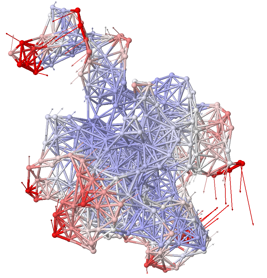
showProtein(oneubi,mode=slowest_mode,data=calcSqFlucts(anm),anim=True,scale=25)

Mode 2

showProtein(oneubi,mode=anm[1].getEigvec(),data=calcSqFlucts(anm),anim=True,amplitude=25)

Compare PCA and ANM

printOverlapTable(pca[:4], anm[:4])

showOverlapTable(pca[:4], anm[:4]);

Mode 1 of PCA

Compare to Mode 2 of ANM

showProtein(oneubi,data=calcSqFlucts(pca[0]),mode=pca[0].getEigvec(),anim=True,amplitude=25)

ProDy Docs and Tutorials

See: http://www.bahargroup.org/prody/tutorials/

Activity

Use ProDy to identify the most variable residues as determined by PCA analysis from NMR ensembles. Given a pdb code (e.g. 2LZ3 or 2L3Y):

• download the structure from the PDB,

• superpose the models of the ensemble (using iterpose with just the alpha carbons),

• calculate the PCA modes (again, just for the alpha carbons).

• Use calcSqFlucts to calculate the magnitude of these fluctuations for each atom.

• Print out the minimum and maximum squared fluctuation value

• Map these values back onto all the atoms of each corresponding residue by setting the B factors (setBetas).

• View this pdb in py3Dmol and color by B factor with reasonable min/max

  • view.setStyle({'cartoon':{'colorscheme':{'prop':'b','gradient':'sinebow','min':0,'max':70}}})