Data analysis principles and pandas
- Storing and analyzing data
- Tidy data principles
- Data handling best practices
- Tidying with
pandas
Questions about data
Why store data?
Analysis -- we want to learn something from the data
- By ourselves, for our own work
- To share with others, along with interpretations
Record keeping
To meet these needs, data should be easy to interpret and easy to use
A case study
... a realistic example of tabular data in the wild: It contains redundant columns, odd variable codes, and many missing values. In short, [this dataset] is messy.
Garrett Grolemund (http://garrettgman.github.io/tidying/)
What does it mean?
This data set describes confirmed cases of tuberculosis (TB) gathered by the WHO
Cases are sorted by country, age, and sex
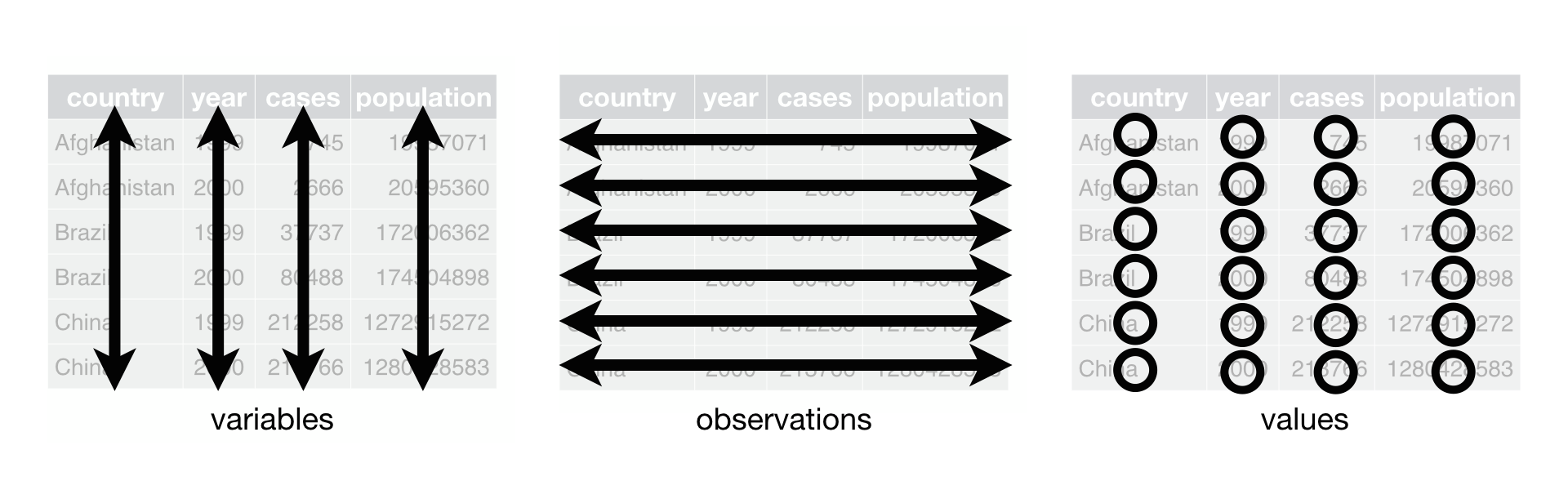
A better way: tidy data
Organizing principles for storing data (see work by Hadley Wickham)
- Each variable forms a column
- Each observation forms a row
- Each value is placed in its own cell
Best practices for data analysis
- Keep a copy of raw data in whatever format it is generated or received
- If at all possible, never manipulate raw data by hand (e.g., copy and paste b/w docs)
- Instead, write and save code to process data
- Record all steps of analysis, including code and versions of software used, so that the entire process is reproducible
Jupyter notebook example
For most packages, __version__ records the version
print('This notebook was prepared using:')

import sys, os
print('python version %s' % sys.version)

import numpy as np
print('numpy version %s' % np.__version__)
More guidelines
- Store paths to data, parameters as (global) variables rather than hard-coding
- Use clear variable names and transparently pass parameters to functions
- Often useful to distinguish global from local variables (e.g., global in ALL_CAPS)
- A neat trick: use dictionaries to pass many named variables at once
my_params = dict(my_number=2, x=7, filename='myfile.dat')
my_function(**my_params)
(Highly condensed) Jupyter notebook example
import my_code

raw_path = 'files/raw/my_data.csv'
processed_path = 'files/processed/processed_data.csv'
output_path = 'files/analysis/my_results.csv'
my_parameter = 7

my_code.process_data(in_file=raw_path, out_file=processed_path, setting=my_parameter)
my_code.generate_results(in_file=processed_path, out_file=output_path)
my_code.plot_results(in_file=output_path)
Comma-separated values (CSV)
- Entries separated by commas
- Rows separated by new line
\ncharacters - The first row gives the names of the variables
- Can be tidy
- Each variable is a column
- Each observation is a row
- Each value in its own cell
country,year,cases,population
Afghanistan,1999,745,19987071
Brazil,2000,2666,172006362
pandas
pandas provides a fast, flexible interface for working with “relational” or “labeled” data that is easy and intuitive
pandas can read and store compressed data automatically, which is a big deal
Especially useful for large data sets with mixed types
Example: the iris dataset in seaborn
Data in pandas is stored in DataFrame objects that can be manipulated in many ways
iris stores measurements of different flower species
%matplotlib inline
import numpy as np
import pandas as pd
import matplotlib.pyplot as plot
import seaborn as sns

df = sns.load_dataset('iris')
df.head(10)
Basic data frame checks
df.columns
len(df)
Showing the relationships between variables
How are petal and sepal lengths related?
sns.jointplot(data=df, x='petal_length', y='sepal_length');
Selecting subsets
print(np.unique(df.species))
Is the relationship between petal and sepal length different for different species?
df_setosa     = df[df.species=='setosa']
df_versicolor = df[df.species=='versicolor']
df_virginica  = df[df.species=='virginica']

sns.jointplot(data=df_setosa, x='petal_length', y='sepal_length');
Visualizing multiple variables at once
Because the data is stored in a simple format, it is easy to quickly relate many variables
sns.pairplot(data=df, hue='species');
A quick test on another data set
planets contains information about recently discovered planets
df = sns.load_dataset('planets')
df.head(10)
How is the year the planet was discovered related to its distance from the solar system?
sns.jointplot(data=df, x='year', y='distance')
plot.yscale('log')
Discovery methods vs. time
sns.catplot(data=df, x='year', kind='count', aspect=4, hue='method');
Example: Tidying the TB dataset
Let's use pandas to load the data set and clean it for analysis
For this and other examples, check here
FYI: iso2 refers to the two-digit country code for different countries
import pandas as pd

df = pd.read_csv('https://raw.githubusercontent.com/hadley/tidy-data/master/data/tb.csv')
df.head(10)
'Melting' the data set
First, extract age range and sex from columns
All values are stored as 'cases'
df = pd.melt(df, id_vars=['iso2', 'year'], value_name='cases', var_name='sex_and_age')
df.head(10)
Parsing the data
# Parse the column names to extract sex, age upper and lower bounds
tmp_df = df['sex_and_age'].str.extract('(\D)(\d+)(\d{2})')

# Add new columns for these variables
tmp_df.columns = ['sex', 'age_lower', 'age_upper']

# Create a single `age` column using `age_lower` and `age_upper`
tmp_df['age'] = tmp_df['age_lower'] + '-' + tmp_df['age_upper']

# Merge the data frames together
df = pd.concat([df, tmp_df], axis=1)

df.head(10)
Reformatting and generating useful variables
# Drop unnecessary columns and rows
df = df.drop(['sex_and_age', 'age_lower', 'age_upper'], axis=1)
df = df.dropna()

# Rename `iso2` to `country`
df = df.rename(index=str, columns={'iso2': 'country'})

# Sort the data frame
df = df.sort_values(['country', 'year', 'sex', 'age'], ascending=True)
df.head(10)
Project
Download the data set (https://mscbio2025-2025.github.io/files/test.csv) and run the steps above, then analyze the data
- What is the trend in TB cases among males in the US over time?
- In 2000, which country had the most TB cases among females?
- Plot the total number of TB cases over time for four countries of your choice (due to large differences in population, you may want to use a log scale)
Download the gene expression data set that we used earlier in the course (https://mscbio2025-2025.github.io/files/Spellman.csv)
- Write a script to convert this data set into a "tidy" format and save it to a new file (
Spellman-tidy.csv) - Read in the new file and plot the expression of the YBR207W gene over time
- Print out the list of genes that have negative expression values at both $t=100$ and $t=200$
Discuss with a neighbor: what kind of data do you encounter in your research? How could you make it easier to store and analyze?
For next time
More data analysis with pandas
Electronic medical records