from IPython.core.display import HTML

def _set_css_style(css_file_path):
   """
   Read the custom CSS file and load it into Jupyter.
   Pass the file path to the CSS file.
   """

   styles = open(css_file_path, "r").read()
   s = '<style>%s</style>' % styles
   return HTML(s)

_set_css_style('rise.css')
Dictionaries, sets, and function fitting
- Dictionaries, sets, and tuples
- Efficient membership testing and hashing
- Curve fitting
- Example data analysis and curve fitting
Dictionary
A dictionary is an unordered collection of (key, value) pairs where the keys are mapped to values
A dictionary object is indexed by the key to get the value
d = dict()
d['key'] = 'value'
d[0] = ['x', 'y', 'z']
print(d)
Initializing dicts
empty = dict()
alsoempty = {}
Specify key:value pairs within curly braces.
example = dict(a=1, b=2)
example
Add new values by indexing with new/existing key
example['a'] = 0
example['z'] = 26
example
Accessing values
example['c'] # keys must exist
Use in to test for membership
'c' in example
if 'c' not in example:
    example['c'] = 0
example
Methods
example.keys()
example.values()
example.items()
What is the output of this function call?
def count(vals):
    counts = {}
    for x in vals:
        counts[x] += 1
    return counts

count(['a','a','b','a','c','b'])
Fixing the function
def count(vals):
    counts = {}
    for x in vals:
        if x not in counts:
            counts[x] = 0
        counts[x] += 1
    return counts

d = count(['a','a','b','a','c','b'])
d
Sets
A set is an unordered collection with no duplicate elements
Basic uses include membership testing and eliminating duplicate entries
Set objects also support mathematical operations like union, intersection, difference, and symmetric difference
stuff = set(['a','b','a','d','x','a','e'])
stuff
Sets are not indexed - use add to insert new elements.
stuff.add('y')
set operations
Efficient membership testing
'y' in stuff
stuff2 = set(['a','b','c'])
print('and', stuff & stuff2) # intersection
print('or', stuff | stuff2)
print('diff', stuff - stuff2)
How many elements are in s?
s = set([1,2,2,3,3,3,4,4,4,4])
s
What is c?
a = set([1,2,2,3])
b = set([2,3,3,4])
c = a & b
c
Tuples
A tuple is an immutable (unchangeable) list
t = tuple([1,2,3])
t
Tuples are initialized the same way as lists, just with parentheses
t = ('x',0,3.0)
l = ['x',0,3.0]
t,l
'%s %d' % ('hello', 3) # second operand of string % operator is tuple
Immutability of tuples
t = ('x', 0, 3.0)
t[2] += 1
Keys
The keys of a dictionary or set should be immutable. Examples of immutable types are numbers, strings, tuples (that contain only immutable objects) and frozensets.
example[(1,2)] = 'a'
example[[1,2]] = 'a'
Dictionaries and sets efficiently store data based on the properties of the key - if the properties of the key can change, then the data structure is broken and the data is not where it should be.
Efficiency
Imagine we have two lists, l1 and l2, and we want do something with the items that are in common in both lists. Here we'll just count them.
def listcount(l1, l2):
    count = 0
    for x in l1:
            if x in l2:
                count += 1
    return count
def setcount(l1, l2):
    count = 0
    s1 = set(l1)
    s2 = set(l2)
    for x in s1:
            if x in s2:
                count += 1
    return count
These two functions generate the same answer if the lists have all distinct elements
Which function is faster?
import time
l1 = list(range(40000))
l2 = list(range(1000,10000))

t0 = time.time()
listcount(l1,l2)
t1 = time.time()
setcount(l1,l2)
t2 = time.time()
print('listcount time: ',t1-t0,'\nsetcount time:  ',t2-t1)
Can you think of another way?
t0 = time.time()
len(set(l1) & set(l2))
t3 = time.time()
print("set intersection time:",t3-t0)
Do not do membership testing on (large) lists
- Lists are ordered by the programmer, which means Python must examine every element to determine (non)membership.
- Dictionaries and sets are unordered so Python can store the contents in a way that makes membership testing efficient (using hashing)
Hashing
The keys of sets and dictionaries must be hashable types. Technically, this means they define methods __eq__ (or __cmp__) and __hash__.
A hash function (__hash__) takes an arbitrary object and produces a number. Objects that are identical (according to __eq__ or __cmp__) must have to the same hash value.
Why is this important?
Accessing an element of an array of elements in memory (random access...) is as simple as computing a memory address (base of array plus offset). This is great if our keys are a dense array of integers (then we have a lookup table).
Hash functions provide a way to quickly index into an array of data even when are keys are arbitray objects.
Hashing
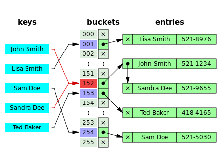
In this figure (from Wikipedia), collisions are resolved through chaining.
With a good hash function and enough buckets, no chain (list) will be more than a few elements long and accessing our data will be constant time (on average). The position of an element in the table is determined by its hash value and the table size.
position = obj.__hash__() % table_size
Hash Functions
A good hash function of an object has the following properties:
- The hash value is fully determined by the object (deterministic)
- The hash function uses all the object's data (if relevant)
- The hash function is uniform (evenly distributes keys across the range)
The range of the hash function is usual the integers ($2^{32}$ or $2^{64}$).
print(hash(3), hash(1435080909832), hash('cat'), hash((3,'cat')))
Takeaway
sets, frozensets, and dicts use hashing to provide extremely efficient membership testing and (for dicts) value lookup
However, you cannot rely on the order of data in these data structures. In fact, the order of items will change as you add and delete
s = set([3,999])
s
s.add(1000)
print(s)
s.update([1001,1002,1003])
print(s)
polyfit takes $x$ values, $y$ values, and degree of polynomial, returns coefficients with least squares fit (highest degree first)
import numpy as np
xvals = np.linspace(-1,2,20)
yvals = xvals**3 + np.random.random(20) #adds random numbers from 0 to 1 to 20 values of xvals
yvals
import matplotlib.pyplot as plt
%matplotlib inline
plt.plot(xvals,yvals,'o');
polyfit
Reminder: $y = x^3$ + noise
deg1 = np.polyfit(xvals,yvals,1)
deg2 = np.polyfit(xvals,yvals,2)
deg3 = np.polyfit(xvals,yvals,3)
deg1
deg2
deg3
poly1d
Construct a polynomial function from coefficients
p1 = np.poly1d(deg1)
p2 = np.poly1d(deg2)
p3 = np.poly1d(deg3)
p1(2),p2(2),p3(2)
p1(0),p2(0),p3(0)
plt.plot(xvals,yvals,'o',xvals,p1(xvals),'-',xvals,p2(xvals),'-',xvals,p3(xvals),'-');
scipy.optimize.curve_fit
Optimize fit to an arbitrary function. Returns optimal values (for least squares) of parameters along with covariance estimate.
Provide python function that takes x value and any parameters
from scipy.optimize import curve_fit

def tanh(x,a,b):
    return b*np.tanh(a+x)

popt, pconv = curve_fit(tanh, xvals, yvals)
popt
plt.plot(xvals,yvals,'o',xvals,popt[1]*np.tanh(popt[0]+xvals)); plt.show()
!head ../files/aff.min
kd contains experimental values while aff.min and aff.score contain computational predictions of the experimental values. Each line has a name and value.
How good are the predictions?
How do we want to load and store the data?
The rows of the provided files are not in the same order.
We only care about points that are in all three files.
Hint: use dictionary to associate names with values.
import numpy as np

def makedict(fname):
    f = open(fname)
    retdict = {}
    for line in f:
        (name,value) = line.split()
        retdict[name] = float(value)
    return retdict

kdvalues = makedict('../files/kd')
scorevalues = makedict('../files/aff.score')
minvalues = makedict('../files/aff.min')

names = []
kdlist = []
scorelist = []
minlist = []
for name in sorted(kdvalues.keys()):
    if name in scorevalues and name in minvalues:
        names.append(name)
        kdlist.append(kdvalues[name])
        scorelist.append(scorevalues[name])
        minlist.append(minvalues[name])

kds = np.array(kdlist)
scores = np.array(scorelist)
mins = np.array(minlist)
How do we want to visualize the data?
Plot experiment value vs. predicted values (two series, scatterplot).
%matplotlib inline
import matplotlib.pylab as plt
plt.plot(kds,scores,'o',alpha=0.5,label='score')
plt.plot(kds,mins,'o',alpha=0.5,label='min')
plt.legend(numpoints=1)
plt.xlim(0,18)
plt.ylim(0,18)
plt.xlabel('Experiment')
plt.ylabel('Prediction')
plt.gca().set_aspect('equal')
plt.show()
Aside: Visualizing dense 2D distributions
seaborn - extends matplotlib to make some hard things easy
import seaborn as sns  # package that sits on top of matplotlib
sns.jointplot(x=kds, y=scores);
sns.jointplot(x=kds, y=scores, kind='hex');
sns.jointplot(x=kds, y=scores, kind='kde');
What is the error?
Average absolute? Mean squared?
print("Scores absolute average error:", np.mean(np.abs(scores-kds)))
print("Mins absolute average error:", np.mean(np.abs(mins-kds)))
print("Scores Mean squared error:", np.mean((scores-kds)**2))
print("Mins Mean squared error:", np.mean((mins-kds)**2))
plt.hist(np.square(kds-mins),bins=25,range=(0,25),density=True)
plt.show()
ave = np.mean(kds)
print("Average experimental value",ave)
print("Error of predicting the average",np.mean(np.square(kds-ave)))
Do the predictions correlate with the observed values?
Compute correlations: np.corrcoef, scipy.stats.pearsonr, scipy.stats.spearmanr
np.corrcoef(kds,scores)
np.corrcoef(kds,mins)
import scipy.stats as stats
stats.pearsonr(kds,scores)
stats.spearmanr(kds,scores)
What is the linear relationship?
fit = np.polyfit(kds,scores,1)
fit
line = np.poly1d(fit) #converts coefficients into function
line(3)
xpoints = np.linspace(0,18,100) #make 100 xcoords
plt.plot(kds,scores,'o',alpha=0.5,label='score')
plt.plot(kds,mins,'o',alpha=0.5,label='min')
plt.xlim(0,18)
plt.ylim(0,18)
plt.xlabel('Experiment')
plt.ylabel('Prediction')
plt.gca().set_aspect('equal')

plt.plot(xpoints,xpoints,'k')
plt.plot(xpoints,line(xpoints),label="fit",linewidth=2)
plt.legend(loc='lower right')
plt.show()
What happens if we rescale the predictions?
Apply the linear fit to the predicted values
f2 = np.polyfit(scores,kds,1)
print("Fit:",f2)
fscores = scores*f2[0]+f2[1]
print("Scores Mean squared error:",np.mean(np.square(scores-kds)))
print("Fit Scores Mean squared error:",np.mean(np.square(fscores-kds)))
plt.plot(kds,scores,'o',alpha=0.5,label='score')
plt.plot(kds,fscores,'o',alpha=0.5,label='fit')
plt.xlim(0,18)
plt.ylim(0,18)
plt.xlabel('Experiment')
plt.ylabel('Prediction')
plt.gca().set_aspect('equal')

plt.plot(xpoints,xpoints)
plt.legend(loc='lower right')
plt.show()
stats.pearsonr(kds,fscores)
For next time
Systems biology modeling (guest lecture by Prof. James Faeder)