Clustering and Dimensionality Reduction

print view
notebook

What is clustering?

Grouping similar objects together based on features describing the objects.

It is used in a lot of different fields.

(e.g. biology, medicine, astronomy, finance, geology, climatology, ...)

Why is clustering important in computational biology?

- Grouping genes, proteins, cells into groups based on expression, structural, or functional similarities.

- Discovering patterns

- Pre-processing step in downstream stream computational analysis.

Assumptions behind clustering

- Biological data has inherent organization and pattern

- Assumption: Similar objects within the data that have similar organization/patterns.

- Goal: Use mathematics and computation to leverage this similarity and group the objects together.

Let's start with a classical example: IRIS dataset

The IRIS dataset contains measurements of 150 iris flowers from 3 species:

• Setosa
• Versicolor
• Virginica

Each flower has 4 features:

• Sepal length (cm)
• Sepal width (cm)
• Petal length (cm)
• Petal width (cm)

import pandas as pd
from sklearn.datasets import load_iris

# Load IRIS dataset
iris = load_iris()

X = iris.data # object features
y = iris.target # object labels

feature_names = iris.feature_names
target_names = iris.target_names

print(X[:5,:]) #print first 5 rows of X
print(y) # print object labels

[[5.1 3.5 1.4 0.2]
 [4.9 3.  1.4 0.2]
 [4.7 3.2 1.3 0.2]
 [4.6 3.1 1.5 0.2]
 [5.  3.6 1.4 0.2]]
[0 0 0 0 0 0 0 0 0 0 0 0 0 0 0 0 0 0 0 0 0 0 0 0 0 0 0 0 0 0 0 0 0 0 0 0 0
 0 0 0 0 0 0 0 0 0 0 0 0 0 1 1 1 1 1 1 1 1 1 1 1 1 1 1 1 1 1 1 1 1 1 1 1 1
 1 1 1 1 1 1 1 1 1 1 1 1 1 1 1 1 1 1 1 1 1 1 1 1 1 1 2 2 2 2 2 2 2 2 2 2 2
 2 2 2 2 2 2 2 2 2 2 2 2 2 2 2 2 2 2 2 2 2 2 2 2 2 2 2 2 2 2 2 2 2 2 2 2 2
 2 2]

print(X.shape)
print(len(y))
print(feature_names)
print(target_names)

(150, 4)
150
['sepal length (cm)', 'sepal width (cm)', 'petal length (cm)', 'petal width (cm)']
['setosa' 'versicolor' 'virginica']

# Create a DataFrame for easier manipulation
df = pd.DataFrame(X, columns=feature_names)
df['species'] = pd.Categorical.from_codes(y, target_names) 

print(df.head())

   sepal length (cm)  sepal width (cm)  petal length (cm)  petal width (cm)  \
0                5.1               3.5                1.4               0.2   
1                4.9               3.0                1.4               0.2   
2                4.7               3.2                1.3               0.2   
3                4.6               3.1                1.5               0.2   
4                5.0               3.6                1.4               0.2   

  species  
0  setosa  
1  setosa  
2  setosa  
3  setosa  
4  setosa  

print(pd.Categorical.from_codes(y, target_names))

['setosa', 'setosa', 'setosa', 'setosa', 'setosa', ..., 'virginica', 'virginica', 'virginica', 'virginica', 'virginica']
Length: 150
Categories (3, object): ['setosa', 'versicolor', 'virginica']

import seaborn as sns
from matplotlib import pyplot as plt
fig1 = plt.figure(figsize=(5, 5))
sns.pairplot(df)

<seaborn.axisgrid.PairGrid at 0x7bd2c87822c0>

<Figure size 500x500 with 0 Axes>

from sklearn.cluster import KMeans
from sklearn.preprocessing import StandardScaler

scaler = StandardScaler()
X_scaled = scaler.fit_transform(X)

kmeans = KMeans(n_clusters=3, init='random', n_init=10, random_state=42)
cluster_labels = kmeans.fit_predict(X_scaled)

cluster_labels_category = pd.Categorical.from_codes(cluster_labels, target_names)
df['cluster'] = cluster_labels_category

sns.pairplot(df,hue='cluster')

<seaborn.axisgrid.PairGrid at 0x7bd2b42468b0>

sns.pairplot(df,hue='species')

<seaborn.axisgrid.PairGrid at 0x7bd2b4247ce0>

from sklearn.metrics import confusion_matrix
conf_matrix = confusion_matrix(y, cluster_labels)

print("Confusion Matrix:")
print("(Rows = True Species, Columns = Predicted Clusters)\n")
conf_df = pd.DataFrame(conf_matrix, 
                       index=target_names,
                       columns=[f'Cluster {i}' for i in range(3)])

print(conf_df)

Confusion Matrix:
(Rows = True Species, Columns = Predicted Clusters)

            Cluster 0  Cluster 1  Cluster 2
setosa             50          0          0
versicolor          0         38         12
virginica           0         14         36

Digression into dimesionality reduction

Representing high-dimensional data using a lower number of features (dimensions) while ensuring that original data’s meaningful properties are still captured

An Example

Principal component analysis finds an orthogonal basis that best represents the variance in the data.

from sklearn.decomposition import PCA

pca = PCA(n_components=2);
X_pca = pca.fit_transform(X_scaled)
#Get cluster centers in PCA
centers_pca = pca.transform(kmeans.cluster_centers_)

fig, axes = plt.subplots(1,2, figsize = (16,5))
scatter1 = axes[0].scatter(X_pca[:,0],X_pca[:,1], c=y, cmap='Set1', s=100, alpha=0.6, edgecolors='black')
axes[0].set_xlabel(f'PC1 ({pca.explained_variance_ratio_[0]*100:.1f}% variance)', fontsize=12)
axes[0].set_ylabel(f'PC2 ({pca.explained_variance_ratio_[1]*100:.1f}% variance)', fontsize=12)
axes[0].set_title('Truth', fontsize=14, fontweight='bold')


scatter2 = axes[1].scatter(X_pca[:,0],X_pca[:,1], c=cluster_labels, cmap='Set1', s=100, alpha=0.6, edgecolors='black')
axes[1].set_xlabel(f'PC1 ({pca.explained_variance_ratio_[0]*100:.1f}% variance)', fontsize=12)
axes[1].set_ylabel(f'PC2 ({pca.explained_variance_ratio_[1]*100:.1f}% variance)', fontsize=12)
axes[1].set_title('Kmeans prediction', fontsize=14, fontweight='bold')

Text(0.5, 1.0, 'Kmeans prediction')

So what is PCA doing

Standardize the dataset

Compute covariance matrix

Compute eigenvalues and eigenvectors

Identify the eigenvectors corresponding to the largest two eigenvalues.

Project data on the two eigenvectors.

import numpy as np
# Compute covariance matrix
cov_matrix = np.cov(X_scaled.T)
print(cov_matrix)

[[ 1.00671141 -0.11835884  0.87760447  0.82343066]
 [-0.11835884  1.00671141 -0.43131554 -0.36858315]
 [ 0.87760447 -0.43131554  1.00671141  0.96932762]
 [ 0.82343066 -0.36858315  0.96932762  1.00671141]]

# Step 4: Compute eigenvalues and eigenvectors
eigenvalues, eigenvectors = np.linalg.eig(cov_matrix)
print(eigenvalues[0:2]/eigenvalues.sum()*100)

[72.96244541 22.85076179]

from matplotlib.pylab import cm
plt.figure(figsize=(16,2))
sns.heatmap(pca.components_,cmap=cm.seismic,yticklabels=['PC1','PC2'],
            square=True, cbar_kws={"orientation": "horizontal"});

Hierarchical clustering

Building a tree-like structure - a hierarchy - of clusters, with

• Each data point starts as its own cluster (Agglomerative/Bottom-up) OR all points start as one cluster (Divisive/Top-down)
• Clusters are progressively merged (or split)
• The result is a nested hierarchy showing relationships at all levels

Linkages

Single Linkage

Complete Linkage

Average Linkage

Ward Linkage

import numpy as np
import matplotlib.pyplot as plt
from sklearn import datasets

# Set random seed for reproducibility
np.random.seed(42)

# Generate datasets
def generate_datasets():
    """Generate various datasets similar to the image"""
    datasets_list = []
    
    # 1. Concentric circles
    noisy_circles = datasets.make_circles(n_samples=300, factor=0.5, noise=0.05)
    datasets_list.append(('Circles', noisy_circles[0], noisy_circles[1]))
    
    # 2. Noisy moons
    noisy_moons = datasets.make_moons(n_samples=300, noise=0.05)
    datasets_list.append(('Moons', noisy_moons[0], noisy_moons[1]))
    
    # 3. Blobs (varied)
    blobs = datasets.make_blobs(n_samples=300, centers=3, cluster_std=0.5, random_state=8)
    datasets_list.append(('Blobs', blobs[0], blobs[1]))
    
    # 4. Anisotropic blobs
    X, y = datasets.make_blobs(n_samples=300, centers=3, random_state=42)
    transformation = [[0.6, -0.6], [-0.4, 0.8]]
    X_aniso = np.dot(X, transformation)
    datasets_list.append(('Anisotropic', X_aniso, y))
    
    # 5. Different variances
    varied = datasets.make_blobs(n_samples=300, centers=3, 
                                  cluster_std=[1.0, 2.5, 0.5], random_state=42)
    datasets_list.append(('Varied', varied[0], varied[1]))
    
    return datasets_list

datasets_list = generate_datasets()
linkage_methods = ['single', 'average', 'complete', 'ward']
fig, axes = plt.subplots(1, len(datasets_list), figsize=(15, 5));
cnt = 0;
for ax in axes:
    ax.scatter(datasets_list[cnt][1][:,0], datasets_list[cnt][1][:,1],
                 color='gray',s=20,alpha=0.7);
    ax.set_title(datasets_list[cnt][0], fontsize=14, fontweight='bold')
    cnt += 1;

colors = ['#1f77b4', '#ff7f0e', '#2ca02c']  # Blue, Orange, Green
fig, axes = plt.subplots(1, len(datasets_list), figsize=(15, 5));
cnt = 0;
for ax in axes:
    for label in datasets_list[cnt][2]:
        mask = datasets_list[cnt][2] == label
        ax.scatter(datasets_list[cnt][1][mask,0], datasets_list[cnt][1][mask,1], c=colors[label.astype('uint8')], s=20,alpha=0.7);
        ax.set_title(datasets_list[cnt][0], fontsize=14, fontweight='bold')
    cnt += 1;

# Hierarchical clustering with different linkage methods
def perform_clustering(X, method='single', n_clusters=3):
    """Perform hierarchical clustering"""
    # Standardize features
    X_scaled = StandardScaler().fit_transform(X)
    
    # Perform hierarchical clustering
    start_time = time.time()
    Z = linkage(X_scaled, method=method)
    elapsed_time = time.time() - start_time
    
    # Get cluster labels
    labels = fcluster(Z, n_clusters, criterion='maxclust')
    
    return labels, elapsed_time

from scipy.cluster.hierarchy import dendrogram, linkage
from scipy.cluster.hierarchy import fcluster
from sklearn.preprocessing import StandardScaler
import time

linkage_methods = ['single', 'average', 'complete', 'ward']
    
fig, axes = plt.subplots(len(datasets_list), len(linkage_methods), 
                             figsize=(16, 18))
    
# Color map
colors = ['#1f77b4', '#ff7f0e', '#2ca02c']  # Blue, Orange, Green
true_clusters=[2,2,3,3,3,1];
cnt=0;
for i, (dataset_name, X, y_true) in enumerate(datasets_list):
    for j, method in enumerate(linkage_methods):
        ax = axes[i, j]
            
        # Perform clustering
        labels, elapsed_time = perform_clustering(X, method=method, n_clusters=true_clusters[cnt])
            
        # Plot the results
        for cluster_id in range(1, 4):
            mask = labels == cluster_id
            ax.scatter(X[mask, 0], X[mask, 1], 
                          c=colors[cluster_id-1], s=20, alpha=0.7,
                          edgecolors='none')
            
        # Remove axes
        ax.set_xticks([])
        ax.set_yticks([])
            
      
        # Add column titles
        if i == 0:
           title = method.replace('_', ' ').title() + ' Linkage'
           ax.set_title(title, fontsize=14, fontweight='bold')
            
        # Add row labels
        if j == 0:
            ax.set_ylabel(dataset_name, fontsize=12, rotation=0, 
                    ha='right', va='center', labelpad=30)
    cnt += 1;
plt.tight_layout()
plt.show()
    

from scipy.cluster.hierarchy import linkage, fcluster, dendrogram

# 1. Load and standardize IRIS data
iris = load_iris()
X = iris.data
scaler = StandardScaler()
X_scaled = scaler.fit_transform(X)

# 2. Perform hierarchical clustering
Z = linkage(X_scaled, method='ward')

# 3. Cut dendrogram to get 3 clusters
clusters = fcluster(Z, t=3, criterion='maxclust') - 1

# 4. Visualize dendrogram
fig, ax = plt.subplots(figsize=(12, 6))

# Create dendrogram
dendrogram(Z, ax=ax, 
           labels=y,  # Color by true species
           color_threshold=0,
           above_threshold_color='gray')

ax.set_title('Hierarchical Clustering Dendrogram (Ward Linkage)', 
             fontsize=14, fontweight='bold')
ax.set_xlabel('Sample Index', fontsize=12)
ax.set_ylabel('Distance (Ward)', fontsize=12)

# Add horizontal line showing where we cut for k=3
ax.axhline(y=6, color='red', linestyle='--', linewidth=2, 
           label='Cut at k=3 clusters')
ax.legend(fontsize=10)
plt.show()

print(f"Created {len(set(clusters))} clusters")
print(f"Cluster sizes: {[sum(clusters == i) for i in range(3)]}")

Created 3 clusters
Cluster sizes: [np.int64(49), np.int64(30), np.int64(71)]

Different types of dimensionality reduction approaches

Linear

• Principal Component Analysis (PCA)
• Linear Discriminant Analysis (LDA)

Non-Linear

• t-distributed stochastic neighbor embedding (t-SNE)
• Uniform manifold approximation and projection (UMAP)

PCA vs LDA

Now let us consider data on a manifold

from sklearn.datasets import make_swiss_roll
import matplotlib.pyplot as plt

points, colors = make_swiss_roll(n_samples=3000, random_state=10);

#Let's plot the Swiss roll
fig = plt.figure(figsize=(6, 6))
ax = fig.add_subplot(111, projection="3d")
fig.add_axes(ax)
ax.scatter(
    points[:, 0], points[:, 1], points[:, 2], c=colors, 
    s=50, alpha=0.5, cmap=plt.cm.Spectral
)
ax.set_title("Swiss Roll")
ax.view_init(azim=-66, elev=10)
#_ = ax.text2D(0.8, 0.05, s="n_samples=1500", transform=ax.transAxes)

#lets perform PCA on the swiss roll
from sklearn.decomposition import PCA
pca_model = PCA(n_components=2)
pca_result = pca_model.fit_transform(points)

plt.figure(figsize=(6, 6))
plt.scatter(pca_result[:, 0], pca_result[:, 1], c=colors, 
            s=50, alpha=0.5, cmap=plt.cm.Spectral)
plt.xlabel('First Principal Component')
plt.ylabel('Second Principal Component')
plt.title('PCA of Swiss Roll')
plt.grid(True)

plt.tight_layout()
plt.show()

# Is the following better 2D projection though?

plt.figure(figsize=(6, 6))
plt.scatter(colors,points[:,1], c=colors, s=50, alpha=0.5, cmap=plt.cm.Spectral)
plt.title('Unwrapping the Swissroll')
plt.grid(True)

plt.tight_layout()
plt.show()

import umap
umap_model = umap.UMAP()
umap_result = umap_model.fit_transform(points, n_neighbors=100, min_dist = .5)

plt.figure(figsize=(6, 6))
plt.scatter(umap_result[:, 0], umap_result[:, 1], c=colors, s=50, alpha=0.5, cmap=plt.cm.Spectral)
plt.xlabel('UMAP 1')
plt.ylabel('UMAP 2')
plt.title('UMAP of Swiss Roll')
plt.grid(True)

plt.tight_layout()
plt.show();

UMAP: Uniform Manifold Approximation & Projection

https://umap-learn.readthedocs.io/en/latest/index.html

Idea: Prioritize respecting local distances in embedding space.

UMAP: Uniform Manifold Approximation & Projection

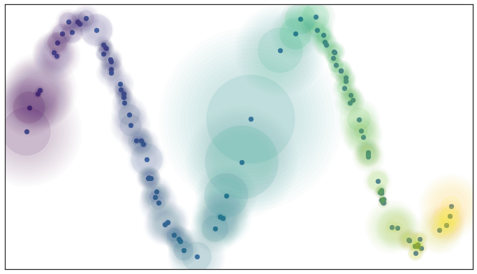
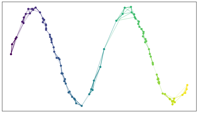
UMAP constructs a $k$-nearest neighbors graph of the data. It uses an approximate stochastic algorithm to do this quickly.

UMAP Parameters

• n_neighbors (15): Number of nearest neighbors to consider. Increase to respect global structure more.
• min_dist (0.1): Minimum distance between points in reduced space. Decrease to have more tightly clustered points.
• metric ("euclidean"): How distance is computed. Can provide user-supplied functions in addition to standard metrics

import numpy as np
import matplotlib.pyplot as plt
from sklearn.datasets import make_moons
from umap import UMAP

# Generate synthetic data
n_samples = 1000
X, y = make_moons(n_samples=n_samples, noise=0.1, random_state=42)
plt.figure(figsize=(6, 6))
plt.scatter(X[:, 0], X[:, 1], c=y, s=10, alpha=0.5, cmap=plt.cm.Spectral)

<matplotlib.collections.PathCollection at 0x7a7e531f0690>

# Set up the plot
fig, axs = plt.subplots(3, 3, figsize=(15, 15))
fig.suptitle("UMAP Parameter Sensitivity", fontsize=16)

# Define parameter ranges
n_neighbors_range = [5, 15, 50]
min_dist_range = [0.0, 0.1, 0.5]

# Generate UMAP projections for different parameter combinations
for i, n_neighbors in enumerate(n_neighbors_range):
    for j, min_dist in enumerate(min_dist_range):
        umap = UMAP(n_neighbors=n_neighbors, min_dist=min_dist, random_state=42, n_jobs=1)
        X_umap = umap.fit_transform(X)
        
        axs[i, j].scatter(X_umap[:, 0], X_umap[:, 1], c=y, cmap=plt.cm.Spectral, s=5)
        axs[i, j].set_title(f'n_neighbors={n_neighbors}, min_dist={min_dist}')
        axs[i, j].set_xticks([])
        axs[i, j].set_yticks([])

plt.tight_layout()
plt.show()

Next time

-RNA seq